
前回の記事はk-means++, x-meansなどのクラスター分析を解説しました。
今回は密度ベースのOPTICSクラスターを解説します。
OPTICSクラスターとは
OPTICS (Ordering Points To Identify the Clustering Structure)は密度ベースのクラスター分析(Density-based Clustering)の手法の一つです。ポイントが集中しているエリアおよび空または疎なエリアによって分離されているエリアを検出します。このアルゴリズムは、空間位置および指定された近傍数までの距離のみに基づいてパターンを自動的に検出します。DBSCANと似ているアルゴリズムになります。そのためクラスター数を決める必要がないアルゴリスムになります。
DBSCAN と OPTICSの検索距離
DBSCAN では、3つの点が存在しています。クラスターの中心、クラスターから到達できるもの、そしてノイズになります。特定のポイントからの検索距離の範囲内でクラスター内にない場合は、そのポイントにはノイズとして他のクラスターだとマークが付けられます。そのためクラスタリングといいつつ外れているものも検出することになります。
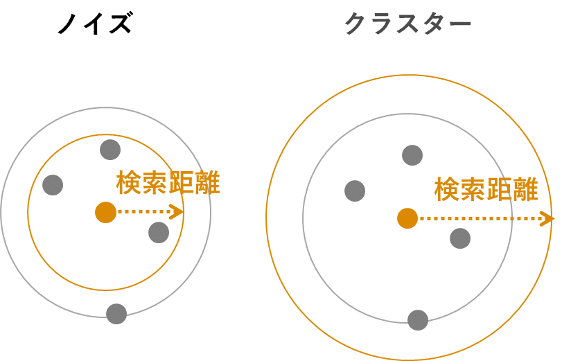
OPTICS の場合、検索距離は中心距離と比較される最大距離として扱われます。マルチスケール OPTICS は、最大到達可能性距離の概念を使用します。この距離は、あるポイントから、検索によってまだ訪問されていない最も近いポイントまでの距離です。

sklearn.cluster.cluster_optics_dbscanでOPTICSクラスターを作成します。scikit-learn 0.21.3が必要です。
pip install -U scikit-learn
ライブラリのロード
%matplotlib inline

from sklearn.cluster import OPTICS, cluster_optics_dbscan
import matplotlib.gridspec as gridspec
import matplotlib.pyplot as plt
import numpy as np
サンプルを作成
np.random.seed(0)

n_points_per_cluster = 250
C1 = [-5, -2] + .8 * np.random.randn(n_points_per_cluster, 2)
C2 = [4, -1] + .1 * np.random.randn(n_points_per_cluster, 2)
C3 = [1, -2] + .2 * np.random.randn(n_points_per_cluster, 2)
C4 = [-2, 3] + .3 * np.random.randn(n_points_per_cluster, 2)
C5 = [3, -2] + 1.6 * np.random.randn(n_points_per_cluster, 2)
C6 = [5, 6] + 2 * np.random.randn(n_points_per_cluster, 2)

X = np.vstack((C1, C2, C3, C4, C5, C6))
モデル作成
clust = OPTICS(min_samples=50, xi=.05, min_cluster_size=.05)

# Run the fit
clust.fit(X)
labels_050 = cluster_optics_dbscan(reachability=clust.reachability_,
                                   core_distances=clust.core_distances_,
                                   ordering=clust.ordering_, eps=0.5)
labels_200 = cluster_optics_dbscan(reachability=clust.reachability_,
                                   core_distances=clust.core_distances_,
                                   ordering=clust.ordering_, eps=2)

space = np.arange(len(X))
reachability = clust.reachability_[clust.ordering_]
labels = clust.labels_[clust.ordering_]
図作成
plt.figure(figsize=(10, 7))
G = gridspec.GridSpec(2, 3)
ax1 = plt.subplot(G[0, :])
ax2 = plt.subplot(G[1, 0])
ax3 = plt.subplot(G[1, 1])
ax4 = plt.subplot(G[1, 2])

# Reachability plot
colors = ['g.', 'r.', 'b.', 'y.', 'c.']
for klass, color in zip(range(0, 5), colors):
    Xk = space[labels == klass]
    Rk = reachability[labels == klass]
    ax1.plot(Xk, Rk, color, alpha=0.3)
ax1.plot(space[labels == -1], reachability[labels == -1], 'k.', alpha=0.3)
ax1.plot(space, np.full_like(space, 2., dtype=float), 'k-', alpha=0.5)
ax1.plot(space, np.full_like(space, 0.5, dtype=float), 'k-.', alpha=0.5)
ax1.set_ylabel('Reachability (epsilon distance)')
ax1.set_title('Reachability Plot')

# OPTICS
colors = ['g.', 'r.', 'b.', 'y.', 'c.']
for klass, color in zip(range(0, 5), colors):
    Xk = X[clust.labels_ == klass]
    ax2.plot(Xk[:, 0], Xk[:, 1], color, alpha=0.3)
ax2.plot(X[clust.labels_ == -1, 0], X[clust.labels_ == -1, 1], 'k+', alpha=0.1)
ax2.set_title('Automatic Clustering\nOPTICS')

# DBSCAN at 0.5
colors = ['g', 'greenyellow', 'olive', 'r', 'b', 'c']
for klass, color in zip(range(0, 6), colors):
    Xk = X[labels_050 == klass]
    ax3.plot(Xk[:, 0], Xk[:, 1], color, alpha=0.3, marker='.')
ax3.plot(X[labels_050 == -1, 0], X[labels_050 == -1, 1], 'k+', alpha=0.1)
ax3.set_title('Clustering at 0.5 epsilon cut\nDBSCAN')

# DBSCAN at 2.
colors = ['g.', 'm.', 'y.', 'c.']
for klass, color in zip(range(0, 4), colors):
    Xk = X[labels_200 == klass]
    ax4.plot(Xk[:, 0], Xk[:, 1], color, alpha=0.3)
ax4.plot(X[labels_200 == -1, 0], X[labels_200 == -1, 1], 'k+', alpha=0.1)
ax4.set_title('Clustering at 2.0 epsilon cut\nDBSCAN')

plt.tight_layout()
plt.show()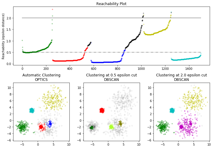
端の黒い部分は、ノイズになります。距離によってクラスタリング数が異なることがわかります。パラメーターとして距離が重要なパラメーターになっていることがわかります。
詳細: