
前回の記事は深層学習について解説しました。
今回はディープラーニングのプーリングレイヤー (Pooling layer)を解説します。
Kerasでは様々なレイヤーが事前定義されており、それらをレゴブロックのように組み合わせてモデルを作成していきます。事前定義されてレイヤーを組み合わせてCNN、LSTM、などのニューラルネットワークを作成します。今回はPoolingレイヤーを説明します。
プーリングレイヤーとは
プーリング層は通常畳込み層(Convolution Layer)の直後に設置されます。
プーリング層は畳み込み層で抽出された特徴の位置感度を若干低下させることで対象とする特徴量の画像内での位置が若干変化した場合でもプーリング層の出力が普遍になるようにします。
画像の空間サイズの大きさを小さくすることで調整するパラメーターの数を減らし、過学習を防止するようです。
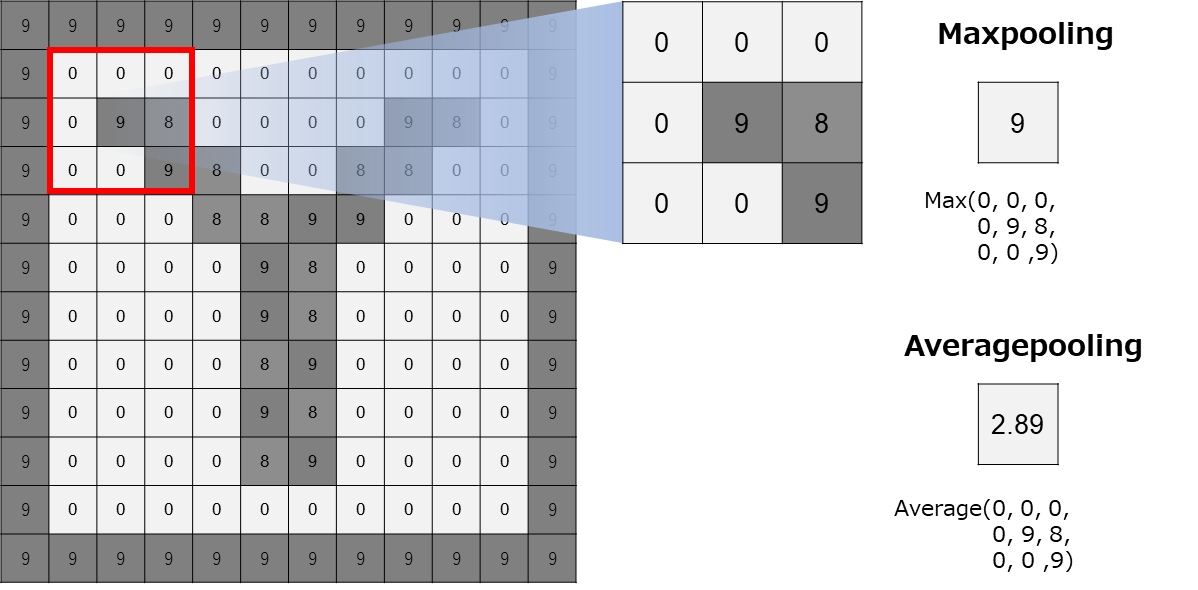
最大プーリング(max pooling)と平均プーリング(average pooling)など様々な種類があるようだが、画像認識への応用では最大プーリングが実用性の面から定番となります。
では、kerasのコートを実験しましょう。
!wget --no-check-certificate \
    https://storage.googleapis.com/mledu-datasets/cats_and_dogs_filtered.zip \
    -O /tmp/cats_and_dogs_filtered.zip
--2019-07-20 07:15:53--  https://storage.googleapis.com/mledu-datasets/cats_and_dogs_filtered.zip
 Resolving storage.googleapis.com (storage.googleapis.com)... 172.217.214.128, 2607:f8b0:4001:c05::80
 Connecting to storage.googleapis.com (storage.googleapis.com)|172.217.214.128|:443... connected.
 HTTP request sent, awaiting response... 200 OK
 Length: 68606236 (65M) [application/zip]
 Saving to: ‘/tmp/cats_and_dogs_filtered.zip’
 /tmp/cats_and_dogs_ 100%[===================>]  65.43M   250MB/s    in 0.3s
 2019-07-20 07:15:59 (250 MB/s) - ‘/tmp/cats_and_dogs_filtered.zip’ saved [68606236/68606236]
import os
import zipfile

local_zip = '/tmp/cats_and_dogs_filtered.zip'
zip_ref = zipfile.ZipFile(local_zip, 'r')
zip_ref.extractall('/tmp')
zip_ref.close()

base_dir = '/tmp/cats_and_dogs_filtered'
train_dir = os.path.join(base_dir, 'train')
validation_dir = os.path.join(base_dir, 'validation')

# Directory
train_cats_dir = os.path.join(train_dir, 'cats')
train_dogs_dir = os.path.join(train_dir, 'dogs')
validation_cats_dir = os.path.join(validation_dir, 'cats')
validation_dogs_dir = os.path.join(validation_dir, 'dogs')

print ('total training cat images:', len(os.listdir(train_cats_dir)))
print ('total training dog images:', len(os.listdir(train_dogs_dir)))
print ('total validation cat images:', len(os.listdir(validation_cats_dir)))
print ('total validation dog images:', len(os.listdir(validation_dogs_dir)))
total training cat images: 1000
total training dog images: 1000
total validation cat images: 500
total validation dog images: 500
from IPython.display import Image

Image('/tmp/cats_and_dogs_filtered/train/cats/cat.115.jpg')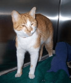
from IPython.display import Image

Image('/tmp/cats_and_dogs_filtered/train/dogs/dog.102.jpg')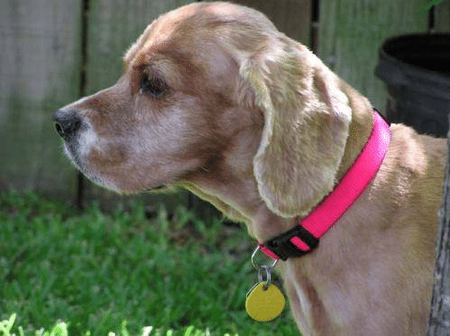
%matplotlib inline
import matplotlib.pyplot as plt
import matplotlib.image as mpimg
from tensorflow.keras import layers
from tensorflow.keras import Model

# Parameters for our graph; we'll output images in a 4x4 configuration
nrows = 4
ncols = 4
# Index for iterating over images
pic_index = 0

# Our input feature map is 150x150x3: 150x150 for the image pixels, and 3 for
# the three color channels: R, G, and B
img_input = layers.Input(shape=(150, 150, 3))

# First convolution extracts 16 filters that are 3x3
# Convolution is followed by max-pooling layer with a 2x2 window
x = layers.Conv2D(16, 3, activation='relu')(img_input)
x = layers.MaxPooling2D(2)(x)
# Second convolution extracts 32 filters that are 3x3
# Convolution is followed by max-pooling layer with a 2x2 window
x = layers.Conv2D(32, 3, activation='relu')(x)
x = layers.MaxPooling2D(2)(x)

# Third convolution extracts 64 filters that are 3x3
# Convolution is followed by max-pooling layer with a 2x2 window
x = layers.Conv2D(64, 3, activation='relu')(x)
x = layers.MaxPooling2D(2)(x)
WARNING: Logging before flag parsing goes to stderr.
W0720 07:16:54.249076 140393464964992 deprecation.py:506] From /usr/local/lib/python3.6/dist-packages/tensorflow/python/ops/init_ops.py:1251: calling VarianceScaling.__init__ (from tensorflow.python.ops.init_ops) with dtype is deprecated and will be removed in a future version.
Instructions for updating:
Call initializer instance with the dtype argument instead of passing it to the constructor
MaxPooling
# Flatten feature map to a 1-dim tensor so we can add fully connected layers
x = layers.Flatten()(x)

# Create a fully connected layer with ReLU activation and 512 hidden units
x = layers.Dense(512, activation='relu')(x)

# Create output layer with a single node and sigmoid activation
output = layers.Dense(1, activation='sigmoid')(x)

model = Model(img_input, output)

model.summary()
Model: "model"
_________________________________________________________________
Layer (type) Output Shape Param #
=================================================================
input_1 (InputLayer) [(None, 150, 150, 3)] 0
_________________________________________________________________
conv2d (Conv2D) (None, 148, 148, 16) 448
_________________________________________________________________
max_pooling2d (MaxPooling2D) (None, 74, 74, 16) 0
_________________________________________________________________
conv2d_1 (Conv2D) (None, 72, 72, 32) 4640
_________________________________________________________________
max_pooling2d_1 (MaxPooling2 (None, 36, 36, 32) 0
_________________________________________________________________
conv2d_2 (Conv2D) (None, 34, 34, 64) 18496
_________________________________________________________________
max_pooling2d_2 (MaxPooling2 (None, 17, 17, 64) 0
_________________________________________________________________
flatten (Flatten) (None, 18496) 0
_________________________________________________________________
dense (Dense) (None, 512) 9470464
_________________________________________________________________
dense_1 (Dense) (None, 1) 513
=================================================================
Total params: 9,494,561
Trainable params: 9,494,561
Non-trainable params: 0
_________________________________________________________________
from tensorflow.keras.optimizers import RMSprop

model.compile(loss='binary_crossentropy',
optimizer=RMSprop(lr=0.001),
metrics=['acc'])

from tensorflow.keras.preprocessing.image import ImageDataGenerator

# All images will be rescaled by 1./255
train_datagen = ImageDataGenerator(rescale=1./255)
test_datagen = ImageDataGenerator(rescale=1./255)

# Flow training images in batches of 20 using train_datagen generator
train_generator = train_datagen.flow_from_directory(
train_dir, # This is the source directory for training images
target_size=(150, 150), # All images will be resized to 150x150
batch_size=20,
# Since we use binary_crossentropy loss, we need binary labels
class_mode='binary')

# Flow validation images in batches of 20 using test_datagen generator
validation_generator = test_datagen.flow_from_directory(
validation_dir,
target_size=(150, 150),
batch_size=20,
class_mode='binary')
# モデル学習
from datetime import datetime

start_time = datetime.now()

history = model.fit_generator(
train_generator,
steps_per_epoch=100, # 2000 images = batch_size * steps
epochs=15,
validation_data=validation_generator,
validation_steps=50, # 1000 images = batch_size * steps
verbose=2)


end_time = datetime.now()
print('Duration: {}'.format(end_time - start_time))
Epoch 1/15
100/100 - 10s - loss: 0.8582 - acc: 0.5525 - val_loss: 0.6455 - val_acc: 0.6120
Epoch 2/15
100/100 - 8s - loss: 0.6376 - acc: 0.6370 - val_loss: 0.6164 - val_acc: 0.6480
Epoch 3/15
100/100 - 8s - loss: 0.5758 - acc: 0.7115 - val_loss: 0.6216 - val_acc: 0.6420
Epoch 4/15
100/100 - 8s - loss: 0.5007 - acc: 0.7610 - val_loss: 0.5871 - val_acc: 0.6950
Epoch 5/15
100/100 - 8s - loss: 0.4226 - acc: 0.8090 - val_loss: 0.6231 - val_acc: 0.6910
Epoch 6/15
100/100 - 8s - loss: 0.3533 - acc: 0.8450 - val_loss: 0.6121 - val_acc: 0.7130
Epoch 7/15
100/100 - 8s - loss: 0.2619 - acc: 0.8900 - val_loss: 0.7127 - val_acc: 0.7310
Epoch 8/15
100/100 - 8s - loss: 0.2003 - acc: 0.9165 - val_loss: 0.7515 - val_acc: 0.7020
Epoch 9/15
100/100 - 8s - loss: 0.1454 - acc: 0.9485 - val_loss: 0.8676 - val_acc: 0.7100
Epoch 10/15
100/100 - 8s - loss: 0.1002 - acc: 0.9600 - val_loss: 0.9935 - val_acc: 0.7320
Epoch 11/15
100/100 - 8s - loss: 0.0768 - acc: 0.9745 - val_loss: 1.6765 - val_acc: 0.6860
Epoch 12/15
100/100 - 8s - loss: 0.0647 - acc: 0.9785 - val_loss: 1.1651 - val_acc: 0.7100
Epoch 13/15
100/100 - 8s - loss: 0.0547 - acc: 0.9835 - val_loss: 1.7297 - val_acc: 0.7250
Epoch 14/15
100/100 - 8s - loss: 0.0481 - acc: 0.9820 - val_loss: 1.7170 - val_acc: 0.7100
Epoch 15/15
100/100 - 8s - loss: 0.0523 - acc: 0.9800 - val_loss: 1.4653 - val_acc: 0.7150
Duration: 0:01:58.872584
# Retrieve a list of accuracy results on training and test data
# sets for each training epoch
acc = history.history['acc']
val_acc = history.history['val_acc']

# Retrieve a list of list results on training and test data
# sets for each training epoch
loss = history.history['loss']
val_loss = history.history['val_loss']

# Get number of epochs
epochs = range(len(acc))

# Plot training and validation accuracy per epoch
plt.plot(epochs, acc)
plt.plot(epochs, val_acc)
plt.title('Training and validation accuracy')

plt.figure()

# Plot training and validation loss per epoch
plt.plot(epochs, loss)
plt.plot(epochs, val_loss)
plt.title('Training and validation loss')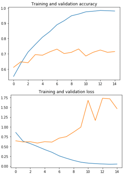
AveragePooling
from tensorflow.keras import layers
from tensorflow.keras import Model

# Our input feature map is 150x150x3: 150x150 for the image pixels, and 3 for
# the three color channels: R, G, and B
img_input = layers.Input(shape=(150, 150, 3))

# First convolution extracts 16 filters that are 3x3
# Convolution is followed by max-pooling layer with a 2x2 window
x = layers.Conv2D(16, 3, activation='relu')(img_input)
x = layers.AveragePooling2D(2)(x)

# Second convolution extracts 32 filters that are 3x3
# Convolution is followed by max-pooling layer with a 2x2 window
x = layers.Conv2D(32, 3, activation='relu')(x)
x = layers.AveragePooling2D(2)(x)

# Third convolution extracts 64 filters that are 3x3
# Convolution is followed by max-pooling layer with a 2x2 window
x = layers.Conv2D(64, 3, activation='relu')(x)
x = layers.AveragePooling2D(2)(x)

# Flatten feature map to a 1-dim tensor so we can add fully connected layers
x = layers.Flatten()(x)

# Create a fully connected layer with ReLU activation and 512 hidden units
x = layers.Dense(512, activation='relu')(x)

# Create output layer with a single node and sigmoid activation
output = layers.Dense(1, activation='sigmoid')(x)

# Create model:
# input = input feature map
# output = input feature map + stacked convolution/maxpooling layers + fully
# connected layer + sigmoid output layer
model = Model(img_input, output)

model.summary()
Model: "model_1"
_________________________________________________________________
Layer (type) Output Shape Param #
=================================================================
input_2 (InputLayer) [(None, 150, 150, 3)] 0
_________________________________________________________________
conv2d_3 (Conv2D) (None, 148, 148, 16) 448
_________________________________________________________________
average_pooling2d (AveragePo (None, 74, 74, 16) 0
_________________________________________________________________
conv2d_4 (Conv2D) (None, 72, 72, 32) 4640
_________________________________________________________________
average_pooling2d_1 (Average (None, 36, 36, 32) 0
_________________________________________________________________
conv2d_5 (Conv2D) (None, 34, 34, 64) 18496
_________________________________________________________________
average_pooling2d_2 (Average (None, 17, 17, 64) 0
_________________________________________________________________
flatten_1 (Flatten) (None, 18496) 0
_________________________________________________________________
dense_2 (Dense) (None, 512) 9470464
_________________________________________________________________
dense_3 (Dense) (None, 1) 513
=================================================================
Total params: 9,494,561
Trainable params: 9,494,561
Non-trainable params: 0
_________________________________________________________________
from tensorflow.keras.optimizers import RMSprop

model.compile(loss='binary_crossentropy',
optimizer=RMSprop(lr=0.001),
metrics=['acc'])

# モデル学習
from datetime import datetime

start_time = datetime.now()

history = model.fit_generator(
train_generator,
steps_per_epoch=100, # 2000 images = batch_size * steps
epochs=15,
validation_data=validation_generator,
validation_steps=50, # 1000 images = batch_size * steps
verbose=2)


end_time = datetime.now()
print('Duration: {}'.format(end_time - start_time))
Epoch 1/15
100/100 - 9s - loss: 0.7698 - acc: 0.5330 - val_loss: 0.6642 - val_acc: 0.6600
Epoch 2/15
100/100 - 8s - loss: 0.6521 - acc: 0.6400 - val_loss: 0.6325 - val_acc: 0.6760
Epoch 3/15
100/100 - 8s - loss: 0.5958 - acc: 0.6825 - val_loss: 0.6463 - val_acc: 0.6620
Epoch 4/15
100/100 - 8s - loss: 0.5251 - acc: 0.7300 - val_loss: 1.0030 - val_acc: 0.5990
Epoch 5/15
100/100 - 8s - loss: 0.4806 - acc: 0.7630 - val_loss: 0.6335 - val_acc: 0.7020
Epoch 6/15
100/100 - 8s - loss: 0.4015 - acc: 0.8170 - val_loss: 0.7374 - val_acc: 0.6810
Epoch 7/15
100/100 - 8s - loss: 0.3235 - acc: 0.8615 - val_loss: 0.7466 - val_acc: 0.6760
Epoch 8/15
100/100 - 8s - loss: 0.2344 - acc: 0.9005 - val_loss: 1.0159 - val_acc: 0.6780
Epoch 9/15
100/100 - 8s - loss: 0.1663 - acc: 0.9360 - val_loss: 0.9899 - val_acc: 0.6720
Epoch 10/15
100/100 - 8s - loss: 0.1050 - acc: 0.9600 - val_loss: 1.5765 - val_acc: 0.6740
Epoch 11/15
100/100 - 8s - loss: 0.1054 - acc: 0.9685 - val_loss: 1.3858 - val_acc: 0.6810
Epoch 12/15
100/100 - 8s - loss: 0.0503 - acc: 0.9855 - val_loss: 2.0894 - val_acc: 0.6990
Epoch 13/15
100/100 - 8s - loss: 0.0585 - acc: 0.9855 - val_loss: 1.5927 - val_acc: 0.6970
Epoch 14/15
100/100 - 8s - loss: 0.0596 - acc: 0.9840 - val_loss: 2.0723 - val_acc: 0.6620
Epoch 15/15
100/100 - 8s - loss: 0.0449 - acc: 0.9885 - val_loss: 2.0870 - val_acc: 0.6830
Duration: 0:01:56.630045
# Retrieve a list of accuracy results on training and test data
# sets for each training epoch
acc = history.history['acc']
val_acc = history.history['val_acc']

# Retrieve a list of list results on training and test data
# sets for each training epoch
loss = history.history['loss']
val_loss = history.history['val_loss']

# Get number of epochs
epochs = range(len(acc))

# Plot training and validation accuracy per epoch
plt.plot(epochs, acc)
plt.plot(epochs, val_acc)
plt.title('Training and validation accuracy')

plt.figure()

# Plot training and validation loss per epoch
plt.plot(epochs, loss)
plt.plot(epochs, val_loss)
plt.title('Training and validation loss')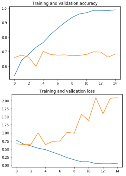
まとめ
Max Pooling
Val_acc 0.73
Duration 1分58秒
Average Pooling
Val_acc 0.70
Duration 1分56秒
今回kerasでプーリングレイヤー (Pooling layer)を紹介しました。犬・猫の画像のデータセットをMaxpoolingとAveragepoolingを実験しました。このデータセットにはMax Poolingの方が制度高いですが、Average Poolingの方が早いと確認しました。