
目次
1. GELU活性化関数の概要
1.1 GELU活性化関数とは
1.2 GELU定義
1.3 GELUの違い
2. 実験
2.1 データロード
2.2 データ前処理
2.3 GELU活性化関数のモデル作成
2.4 ReLU活性化関数のモデル作成
2.5 まとめ
1. GELU活性化関数の概要
1.1 GELU活性化関数とは
GELU活性化関数は、Gaussian Error Linear Unit functionsの略称です。GELUはOpenAI GPTやBERTなどの有名なモデルで使われている活性化関数です。
GELUはReLU、ELU、PReLUなどのアクティベーションにより、シグモイドよりも高速で優れたニューラルネットワークの収束が可能になったと言われています。コツとしては、Dropoutに似た要素を入れている事です。Dropoutとは、いくつかのアクティベーションに0をランダムに乗算することにより、モデルを頑強します。
1.2 GELU定義
Geluは以下のように定義されます。
Computes gaussian error linear:

approximateがFalse場合は、

approximateがTrue場合は、
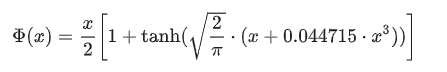
論文:https://arxiv.org/abs/1606.08415
1.3 GELUの違い
GELUとReLUとELUは非凸(non-convex)、非単調(non-monotonic)関数ですが、GELUは正の領域で線形ではなく、曲率があります。
GELUは単調増加ではありません。
GELUは確率的な要素を加味しています(Dropout)。

ライブラリ:
Tensorflow/Keras
https://www.tensorflow.org/addons/api_docs/python/tfa/activations/gelu#returns
PyTorch
https://pytorch.org/docs/stable/generated/torch.nn.GELU.html
2. 実験
環境:Colab
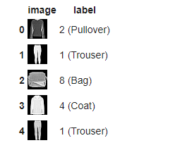
データセット:tensorflowのfashion_mnist
fashion_mnistのデータセットは60,000枚の28×28,Tシャツ/トップス、ズボン、などのプルオーバー10個のファッションカテゴリの白黒画像と10,000枚のテスト用画像データセット。
モデル:GELU活性化関数のDenseモデル、ReLU活性化関数のDenseモデル
モデル評価:Accuracy
2.1 データロード
ライブラリインポート
| import tensorflow as tf import tensorflow_datasets as tfds |
データロード
| (ds_train, ds_test), ds_info = tfds.load( ‘fashion_mnist’, split=[‘train’, ‘test’], shuffle_files=True, as_supervised=True, with_info=True, ) |
データセットの情報を確認します。
– 学習:60,000枚の28×28画像データ
– テスト:10,000枚の28×28画像データ
– 10個のクラス
| builder = tfds.builder(‘fashion_mnist’) info = builder.info print(info) |
tfds.core.DatasetInfo(
name=’fashion_mnist’,
version=3.0.1,
description=’Fashion-MNIST is a dataset of Zalando’s article images consisting of a training set of 60,000 examples and a test set of 10,000 examples. Each example is a 28×28 grayscale image, associated with a label from 10 classes.’,
homepage=’https://github.com/zalandoresearch/fashion-mnist‘,
features=FeaturesDict({
‘image’: Image(shape=(28, 28, 1), dtype=tf.uint8),
‘label’: ClassLabel(shape=(), dtype=tf.int64, num_classes=10),
}),
total_num_examples=70000,
splits={
‘test’: 10000,
‘train’: 60000,
},
supervised_keys=(‘image’, ‘label’),
citation=”””@article{DBLP:journals/corr/abs-1708-07747,
author = {Han Xiao and
Kashif Rasul and
Roland Vollgraf},
title = {Fashion-MNIST: a Novel Image Dataset for Benchmarking Machine Learning
Algorithms},
journal = {CoRR},
volume = {abs/1708.07747},
year = {2017},
url = {http://arxiv.org/abs/1708.07747},
archivePrefix = {arXiv},
eprint = {1708.07747},
timestamp = {Mon, 13 Aug 2018 16:47:27 +0200},
biburl = {https://dblp.org/rec/bib/journals/corr/abs-1708-07747},
bibsource = {dblp computer science bibliography, https://dblp.org}
}”””,
redistribution_info=,
)
理画像データを表示します。
| tfds.as_dataframe(ds_train .take(5), ds_info) |
2.2 データ前処理
学習パイプラインを作成します。データ正規化を行います。
| # Build train pipeline def normalize_img(image, label): “””Normalizes images: `uint8` -> `float32`.””” return tf.cast(image, tf.float32) / 255., label ds_train = ds_train.map( normalize_img, num_parallel_calls=tf.data.experimental.AUTOTUNE) ds_train = ds_train.cache() ds_train = ds_train.shuffle(ds_info.splits[‘train’].num_examples) ds_train = ds_train.batch(128) ds_train = ds_train.prefetch(tf.data.experimental.AUTOTUNE) |
テストパイプラインを作成します。
| # Build evaluation pipeline
ds_test = ds_test.map( normalize_img, num_parallel_calls=tf.data.experimental.AUTOTUNE) ds_test = ds_test.batch(128) ds_test = ds_test.cache() ds_test = ds_test.prefetch(tf.data.experimental.AUTOTUNE) |
2.3 GELU活性化関数のモデル作成
GELU活性化関数のモデルを作成します。
tf.keras.layers.Dense(128,activation=’gelu’) を設定します。
| # Create and train the model
model = tf.keras.models.Sequential([ tf.keras.layers.Flatten(input_shape=(28, 28)), tf.keras.layers.Dense(128,activation=’gelu’), tf.keras.layers.Dense(10) ])
model.compile( optimizer=tf.keras.optimizers.Adam(0.001), loss=tf.keras.losses.SparseCategoricalCrossentropy(from_logits=True), metrics=[tf.keras.metrics.SparseCategoricalAccuracy()], )
history = model.fit( ds_train, epochs=15, validation_data=ds_test, ) |
Epoch 1/15
469/469 [==============================] – 10s 7ms/step – loss: 0.7374 – sparse_categorical_accuracy: 0.7525 – val_loss: 0.4719 – val_sparse_categorical_accuracy: 0.8319
…
Epoch 15/15
469/469 [==============================] – 2s 4ms/step – loss: 0.2171 – sparse_categorical_accuracy: 0.9212 – val_loss: 0.3223 – val_sparse_categorical_accuracy: 0.8885
モデルを確認します。
| model.summary() |
Model: “sequential_10”
_________________________________________________________________
Layer (type) Output Shape Param #
=================================================================
flatten_10 (Flatten) (None, 784) 0
_________________________________________________________________
dense_20 (Dense) (None, 128) 100480
_________________________________________________________________
dense_21 (Dense) (None, 10) 1290
=================================================================
Total params: 101,770
Trainable params: 101,770
Non-trainable params: 0
_________________________________________________________________
モデルを評価します。
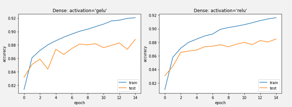
| # plotting the metrics
import matplotlib.pyplot as plt
plt.plot(history.history[‘sparse_categorical_accuracy’]) plt.plot(history.history[‘val_sparse_categorical_accuracy’]) plt.title(‘model accuracy’) plt.ylabel(‘accuracy’) plt.xlabel(‘epoch’) plt.title(“Dense: activation=’gelu'”) plt.legend([‘train’, ‘test’], loc=’lower right’) plt.show() |

2.4 ReLU活性化関数のモデル作成
ReLU活性化関数のモデルを作成します。
tf.keras.layers.Dense(128,activation=’relu’を作成します。
| # Create and train the model
model = tf.keras.models.Sequential([ tf.keras.layers.Flatten(input_shape=(28, 28)), tf.keras.layers.Dense(128,activation=’relu’), tf.keras.layers.Dense(10) ]) model.compile( optimizer=tf.keras.optimizers.Adam(0.001), loss=tf.keras.losses.SparseCategoricalCrossentropy(from_logits=True), metrics=[tf.keras.metrics.SparseCategoricalAccuracy()], ) history = model.fit( ds_train, epochs=15, validation_data=ds_test, ) |
Epoch 1/15
469/469 [==============================] – 2s 4ms/step – loss: 0.7410 – sparse_categorical_accuracy: 0.7499 – val_loss: 0.4667 – val_sparse_categorical_accuracy: 0.8307
…
Epoch 15/15
469/469 [==============================] – 2s 4ms/step – loss: 0.2236 – sparse_categorical_accuracy: 0.9171 – val_loss: 0.3291 – val_sparse_categorical_accuracy: 0.8848
モデル評価
| # plotting the metrics
import matplotlib.pyplot as plt
plt.plot(history.history[‘sparse_categorical_accuracy’]) plt.plot(history.history[‘val_sparse_categorical_accuracy’]) plt.title(‘model accuracy’) plt.ylabel(‘accuracy’) plt.xlabel(‘epoch’) plt.title(“Dense: activation=’relu'”) plt.legend([‘train’, ‘test’], loc=’lower right’) plt.show() |
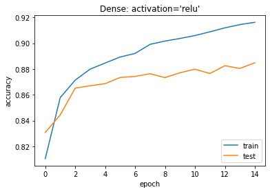
2.5 まとめ
Fashion_mnistのデータセットで、GELU活性化関数のDenseモデルとReLU活性化関数のDenseモデルを作成しました。モデル精度があまり変わらないが、ReLUのモデルの方が安定の結果になりました。

担当者:KW
バンコクのタイ出身 データサイエンティスト
製造、マーケティング、財務、AI研究などの様々な業界にPSI生産管理、在庫予測・最適化分析、顧客ロイヤルティ分析、センチメント分析、SaaS、PaaS、IaaS、AI at the Edge の環境構築などのスペシャリスト