Statsmodelsでの回帰分析

前回の記事は線形回帰を解説しました。
回帰分析の説明はこの記事を参考してください。
線形回帰

回帰分析を行うとき、 Scikit-learn と Statsmodelsのライブラリをよく使います。前回はScikit-learnで回帰分析を行いました。今回はScikit-learnとStatsmodelsのライブラリを比較して、回帰分析を解説・実験します。

１．ライブラリ

1.1 Scikit-learnの回帰分析

sklearn.linear_model.LinearRegression(fit_intercept=True, normalize=False, copy_X=True, n_jobs=None)

パラメータ設定：
fit_intercept : boolean, optional, default True:
False に設定すると切片を求める計算を含めません。

normalize : boolean, optional, default False:
True に設定すると、説明変数を事前に正規化します。

copy_X : boolean, optional, default True：
メモリ内でデータを複製してから実行するかどうか。

n_jobs : int or None, optional (default=None)
計算に使うジョブの数。-1 に設定すると、すべての CPU を使って計算します。

1.2 Statsmodelsの回帰分析

statsmodels.regression.linear_model.OLS(formula, data, subset=None)

アルゴリズムのよって、パラメータを設定します。
・OLS Ordinary Least Squares 普通の最小二乗法
・WLS Weighted Least Squares 加重最小二乗法
・GLS Generalized Least Squares 一般化最小二乗法

モデル式の文法
R-styleの共用を考えています。
モデル式の例：
y ~ x 回帰モデル，yはxにより説明される
y ~ x1 + x2　重回帰モデル，yは，独立変数 x1 と x2 により説明される
y ~ 1 + x1 + x2　y は，(切片 / intercept と）x1，x2 で説明される
質的変数の場合はN-1の変数になります。

data　はpandasのデータフレームです。

2．コード・実験　

概要：
データセット：Duncan’s Occupational Prestige Data：Duncanは、45行と4列があり、1950年の米国の職業の威信およびその他の特性に関するデータセットです。

環境：google colab Python3 GPU
ライブラリ：　Statsmodels
pip install -U statsmodels
モデル：
実験：重回帰分析
モデル評価：R2

2.1 データ準備

ライブラリ

import matplotlib.pyplot as plt
import seaborn as sns; sns.set()
import numpy as np
import statsmodels.api as sm
from statsmodels.formula.api import ols

データセットロード

df = sm.datasets.get_rdataset("Duncan", "carData", cache=True).data
df.head()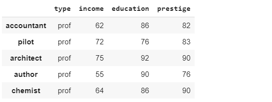

グラフ作成

import matplotlib.pyplot as plt
import matplotlib.gridspec as gridspec

x1 = df.type
x2 = df.income
x3 = df.education
y = df.prestige

fig = plt.figure(figsize=(8,5))

plt.subplot(2,2,1)
plt.plot(x1, y, 'o')
plt.title("type vs prestiage")

plt.subplot(2,2,2)
plt.plot(x2, y, 'o')
plt.title("income vs prestiage")

plt.subplot(2,2,3)
plt.plot(x3, y, 'o')
plt.title("education vs prestiage")

plt.tight_layout()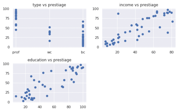

2.2 Sklearnの回帰分析

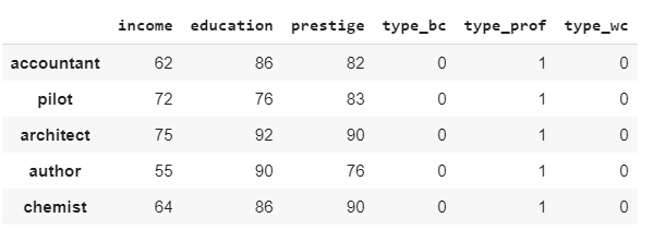
ダミー変数に変更
ダミー変数の詳細は下記の記事をご覧ください。
ダミー変数に変換　【One-Hotエンコーディング】

import pandas as pd

df2 = pd.get_dummies(df)
df2.head()

Sklearnの回帰分析の学習

from sklearn.linear_model import LinearRegression

x = df2.loc[:, df2.columns != 'prestige']
y = df2[['prestige']]

reg_mod = LinearRegression(fit_intercept=True)
reg_mod.fit(x, y)

print(" r2: ", reg_mod.score(x, y))
print(" Coef: ", reg_mod.coef_[0])
print(" intercept: ", reg_mod.intercept_[0])

r2: 0.9130657009984509
Coef: [ 0.5975465 0.34531933 -0.66546001 15.99205339 -15.32659337]
intercept: 0.48043218310085223

2.3 Statsmodelsの回帰分析

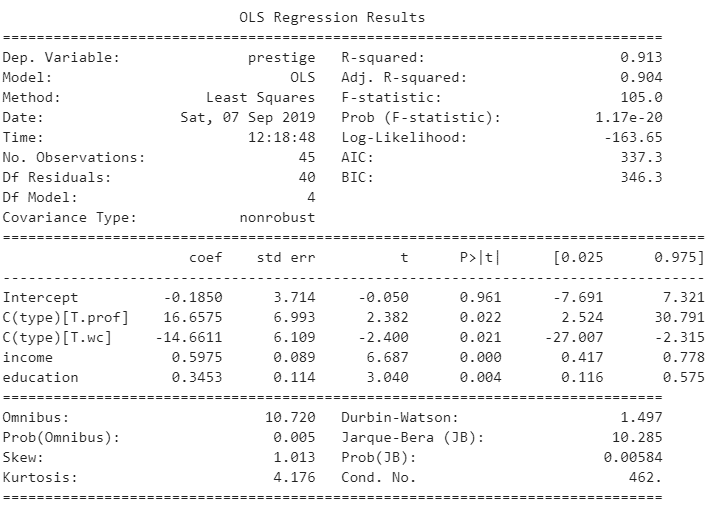
olsmod = ols(formula="prestige ~ C(type) + income + education", data=df).fit()
print(olsmod.summary())

2.4 結果の説明

結果を確認すると、モデルの係数a（T.prof）とモデルの係数b（T.wc）とモデルの係数c（income）と　係数d（education）と定数e（const）はそれぞれ、+16.65, -14.66, +0.59, +0.34, -0.18となることが分かります。よって、このモデルは以下の数式で表すことができます。
［prestige］＝［T.prof］×16.6575 -［T.wc］×14.6611 +［income］×0.5975 +［education］×0.3453 –0.1850

決定係数（R-squared: 0.913）は90％以上であり、よく当てはまっているといえます。
F検定（F-stat: 105, p-value: 1.17e-20）が十分に大きく、有意確率（p-value）も十分に小さいので、モデル全体として妥当であると判断できます。
t検定（係数1 T.prof:t-stat= 2.382、p-value=0.022
係数1 T.wc:t-stat= -2.400、p-value=0.021
係数1 income:t-stat= 6.687、p-value=0.000、
係数2 education:t-stat= 3.040、p-value=0.004、
定数 const:t-stat= -0.050、p-value=0.961）
係数T.prof、係数T.wc、係数income、係数education、定数constの有意確率双方とも十分に小さい値であり係数、定数とも妥当であると判断できます。

summaryのレポートを出力しなくて、特定の値を出力することができます。

print('Parameters: ', olsmod.params)
print('R2: ', olsmod.rsquared)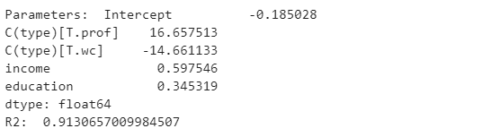

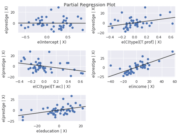
3. Partial Regression Plots

fig = plt.figure(figsize=(8,6))
fig = sm.graphics.plot_partregress_grid(olsmod, fig=fig)
plt.tight_layout()

4. まとめ

今回はPythonのSci-kit learnとStatsmodelsのライブラリで重回帰分析を行いました。Statsmodelsのライブラリは自動でダミー変数を変換し、詳細の結果ができるし、グラフも簡単に作成してもるし、統計量が多いため統計解析に有利なライブラリです。

目次：

１．ライブラリ

1.1 Scikit-learnの回帰分析

1.2 Statsmodelsの回帰分析

2．コード・実験

2.1 データ準備

2.2 Sklearnの回帰分析

2.3 Statsmodelsの回帰分析

2.4 結果の説明

4. まとめ

2．コード・実験　