
Table of Contents
1. What is Survival Analysis?
2. Sample
3. Code (Experiment)
_3.1 Kaplan-Meier fitter
_3.2 Kaplan-Meier fitter Based on Different Groups.
_3.3 Log-Rank-Test
1. What is Survival Analysis?
Survival analysis is a branch of statistics for analyzing the expected duration of time until one or more events happen, such as a death in biological organisms and failure of mechanical systems.
For instance, how can Survival Analysis be useful to analyze the ongoing COVID-19 pandemic data?
・We can find the number of days until patients showed COVID-19 symptoms.
・We can find for which age group it is deadlier.
・We can find which treatment has the highest survival probability.
・We can find whether a person’s sex has a significant effect on their survival time?
・We can find the median number of days of survival for patients.
・We can find which factor has more impact on patients’ survival.
Survival time and type of events in cancer studies
Survival Time: It is usually referred to as an amount of time until when a subject is alive or actively participates in a survey.
There are three main types of events in survival analysis:
1) Relapse: Relapse is defined as a deterioration in the subject’s state of health after a temporary improvement.
2) Progression: Progression is defined as the process of developing or moving gradually towards a more advanced state. It basically means that the health of the subject under observation is improving.
3) Death: Death is defined as the destruction or the permanent end of something. In our case, death will be our event of interest.
Censoring
As we discussed above, survival analysis focuses on the occurrence of an event of interest. The event of interest can be anything like birth, death, or retirement. However, there is still a possibility that the event we are interested in does not occur. Such observations are known as censored observations.
There are three types of censoring:
Right Censoring: The subject under observation is still alive. In this case, we cannot have our timing when our event of interest (death) occurs.
Left Censoring: In this type of censoring, the event cannot be observed for any reason. It may also include the event that occurred before the experiment started, such as the number of days from birth when the kid started walking.
3) Interval Censoring: In this type of data censoring, we only have data for a specific interval, so it is possible that the event of interest does not occur during that time.
2. Use cases
Medical
・Survival timeline Analysis
・Recovery time Analysis
Production
・Machine life Analysis
・Production line Analysis
・Production critical Analysis
・Maintenance Analysis
Business
・ Analysis of warranty claim period
・ Leads to sales time analysis
・ Analysis of sales staff for the first sales analysis
3. Code (Experiment)
Environment:Google Colab
Library:lifelines
Survival analysis was originally developed and applied heavily by the actuarial and medical community. Its purpose was to answer why are events occurring now versus later under uncertainty (where events might refer to deaths, disease remission, etc.). This is great for researchers who are interested in measuring lifetimes: they can answer questions like what factors might influence deaths?
Reference:https://lifelines.readthedocs.io/en/latest/
Dataset:NCCTG Lung Cancer Data
The North Central Cancer Treatment Group (NCCTG) data set records the survival of patients with advanced lung cancer, together with assessments of the patients’ performance status measured either by the physician and by the patients themselves. The goal of the study was to determine whether patients’ self-assessment could provide prognostic information complementary to the physician’s assessment. The data set contains 228 patients, including 63 patients that are right censored (patients that left the study before their death).
Reference:http://www-eio.upc.edu/~pau/cms/rdata/doc/survival/lung.html
3.1 Kaplan-Meier
Library
| !pip install lifelines |
Import Library
| import numpy as np import pandas as pd import matplotlib.pyplot as plt import urllib from urllib import request import lifelines from lifelines import KaplanMeierFitter
print(‘lifelines version: ‘, lifelines.__version__) |
lifelines version: 0.25.5
Download data
| csv_src = “http://www-eio.upc.edu/~pau/cms/rdata/csv/survival/lung.csv” csv_path = ‘lung.csv’ urllib.request.urlretrieve(csv_src, csv_path) |
Create dataframe
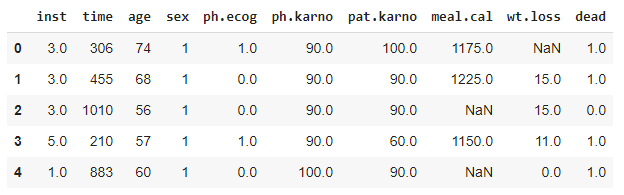
| df = pd.read_csv(csv_path)
# Precessing df.loc[df.status == 1, ‘dead’] = 0 df.loc[df.status == 2, ‘dead’] = 1 df = df.drop([‘Unnamed: 0’, ‘status’], axis=1)
df.head() |
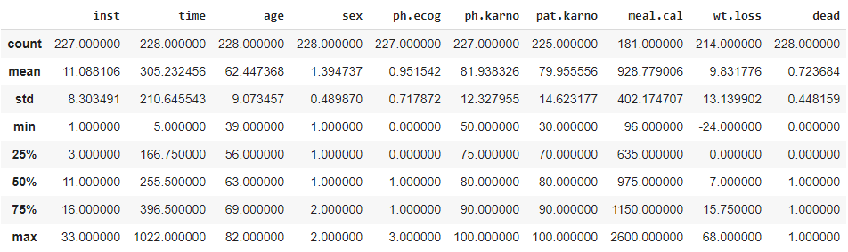
Get statistical info
| df.describe() |
Kaplan-Meier-Fitter
| # Kaplan-Meier-Fitter kmf = KaplanMeierFitter() kmf.fit(durations = df.time, event_observed = df.dead)
|
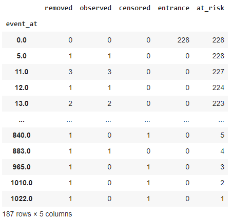
Event table:
- a) event_at: It stores the value of the timeline for our dataset. I.e., when was the patient observed in our experiment or when was the experiment conducted. It can be several minutes, days, months, years, and others. In our case, it is going to be for many days. It stores the value of survival days for the subjects.
- b) at_risk: It stores the number of current patients under observation. In the beginning, it will be the total number of patients we are going to observe in our experiment. If new patients are added at a particular time, then we have to increase their value accordingly. Therefore:
Figure 19: Analyzing at_risk variable. | Survival Analysis with Python Tutorial
Figure 19: at_risk variable formula.
- c) entrance: It stores the value of new patients in a given timeline. It is possible that while experimenting, other patients are also diagnosed with the disease. To account for that, we have the entrance column.
- d) censored: Our ultimate goal is to find the survival probability for a patient. At the end of the experiment, if the person is still alive, we will add him/her to the censored category. We have already discussed the types of censoring.
- e) observed: It stores the value of the number of subjects that died during the experiment. From a broad perspective, these are the people who met our event of interest.
- f) removed: It stores the values of patients that are no longer part of our experiment. If a person dies or is censored, then he/she falls into this category. In short, it is an addition of the data in the observed and censored category.
| kmf.event_table |
Calculating the probability of survival for individual timelines:
Let’s first see the formula for calculating the survival of a particular person at a given time.
Calculating the probability of survival for individual timelines:
Let’s first see the formula for calculating the survival of a particular person at a given time.
![]()
![]()
| # Calculate survival probability for given time
print(“Survival probablity for t=0: “, kmf.predict(0)) print(“Survival probablity for t=5: “, kmf.predict(5)) print(“Survival probablity for t=11: “, kmf.predict(11)) print(“Survival probablity for t=840: “, kmf.predict(840))
print(kmf.predict([0,5,11,840])) |
Survival probablity for t=0: 1.0
Survival probablity for t=5: 0.9956140350877193
Survival probablity for t=11: 0.9824561403508766
Survival probablity for t=840: 0.06712742409441387
0 1.000000
5 0.995614
11 0.982456
840 0.067127
Name: KM_estimate, dtype: float64
survial full list
| # Get survial full list print(kmf.survival_function_) |
KM_estimate
timeline
0.0 1.000000
5.0 0.995614
11.0 0.982456
12.0 0.978070
13.0 0.969298
… …
840.0 0.067127
883.0 0.050346
965.0 0.050346
1010.0 0.050346
1022.0 0.050346
[187 rows x 1 columns]
survival graph curve
| # Plot the survival graph
kmf.plot() plt.title(“Kaplan-Meier”) plt.xlabel(“Number o days”) plt.ylabel(“Probablity of survival”) plt.show()
|

survival time median
| # Get survival time median
survival_time_median = kmf.median_survival_time_ print(” The median survial time: “, survival_time_median) |
The median survial time: 310.0
survival function with confidence interval
| # Plot survival function with confidence interval
survival_confidence_interval = kmf.confidence_interval_survival_function_
plt.plot(survival_confidence_interval[‘KM_estimate_lower_0.95’], label=”Lower”) plt.plot(survival_confidence_interval[‘KM_estimate_upper_0.95’], label=”Upper”) plt.title(“Survival Function with confidence interval”) plt.xlabel(“Number of days”) plt.ylabel(“Survial Probablity”) plt.legend() plt.show()
|

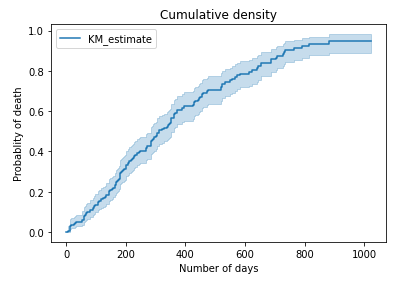
Cumulative survival
| # Cumulative survival cumu_surv = kmf.cumulative_density_
# Plot cumulative density kmf.plot_cumulative_density() plt.title(“Cumulative density”) plt.xlabel(“Number of days”) plt.ylabel(“Probablity of death”) plt.show()
|
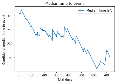
Median survival
| # Median time left for event
median_time_to_event = kmf.conditional_time_to_event_ plt.plot(median_time_to_event, label = “Median time left”) plt.title(“Median time to event”) plt.xlabel(“Total days”) plt.ylabel(“Conditional median time to event”) plt.legend() plt.show() |
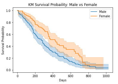
3.2 Kaplan-Meier Estimator with groups
Until now, we saw how we could find the survival probability and hazard probability for all of our observations. Now it is time to perform some analysis on our data to determine whether there is any difference in survival probability if we divide our data into groups based on specific characteristics. Let’s divide our data into two groups based on sex: Male and Female. Our goal here is to check is there any significant difference in survival rate if we divide our dataset based on sex. Later in this tutorial, we will see on what basis do we divide the data into groups.
| # KM for Male and Female
kmf_m = KaplanMeierFitter() kmf_f = KaplanMeierFitter() Male = df.query(“sex == 1”) Female = df.query(“sex == 2″) kmf_m.fit(durations=Male.time, event_observed=Male.dead, label=”Male”) kmf_f.fit(durations=Female.time, event_observed=Female.dead, label=”Female”) |
survival function comparison
| # Plot survival function
kmf_m.plot() kmf_f.plot() plt.title(“KM Survival Probaility: Male vs Female”) plt.xlabel(“Days”) plt.ylabel(“Survival Probability”) plt.show()
|
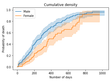
cumulative density comparison
| # Plot cumulative density
kmf_m.plot_cumulative_density() kmf_f.plot_cumulative_density() plt.title(“Cumulative density”) plt.xlabel(“Number of days”) plt.ylabel(“Probablity of death”) plt.show()
|
3.3 Log-Rank Test:
The log-rank test is a hypothesis test that is used to compare the survival distribution of two samples.
Goal: Our goal is to see if there is any significant difference between the groups being compared.
Null Hypothesis: The null hypothesis states that there is no significant difference between the groups being studied. If there is a significant difference between those groups, then we have to reject our null hypothesis.
| from lifelines.statistics import logrank_test
time_m = Male.time event_m = Male.dead
time_f = Female.time event_f = Female.dead
results = logrank_test(time_m, time_f, event_m, event_f) results.print_summary() print(“P-value: “, results.p_value)
|
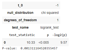
Less than (5% = 0.05) P-value means there is a significant difference between the groups we compared. We can partition our groups based on their sex, age, race, treatment method, and others.
We have compared the survival distributions of two different groups using the famous statistical method, the Log-rank test. Here we can notice that the p-value is 0.00131 (<0.005) for our groups, which denotes that we must reject the null hypothesis and admit that the survival function for both groups is significantly different.

担当者:HM
香川県高松市出身 データ分析にて、博士(理学)を取得後、自動車メーカー会社にてデータ分析に関わる。その後コンサルティングファームでデータ分析プロジェクトを歴任後独立 気が付けばデータ分析プロジェクトだけで50以上担当
理化学研究所にて研究員を拝命中 応用数理学会所属