RandomForestのdtreevizで決定木の可視化

1. dtreeviz 決定木の可視化

dtreevizは決定木関係のアルゴリズム結果を、可視化するライブラリです。対応ライブラリーとしては、scikit-learn, XGBoost, Spark MLlib, LightGBMにおいて利用できます。

Dtreevizは複数プラットフォームに対応されています。

pip install dtreeviz # sklearn

pip install dtreeviz[xgboost] # XGBoost

pip install dtreeviz[pyspark] # pyspark

pip install dtreeviz[lightgbm] # LightGBM

dtreevizライブラリ：https://github.com/parrt/dtreeviz

dtreeviz関数

tree_model	決定木のモデル
X_train	説明変数データ
y_train	目的変数データ
feature_names	X_trainの各特徴量名
target_name	目的変数の名前
class_names	(分類木の時必須)各クラスに対応する名前
precision	特徴量の境界値を表示する小数点以下の桁数
orientation	木が分岐する方向 TD: top-down or LR: left-right
show_root_edge_labels	ルートからノードへの分岐の値関係を表示するか
show_node_labels	ノード番号を表示するか
fancy	特徴量の決定境界を可視化するか
histtype	分類木の時、ヒストグラムの表示形式
X	推論過程を可視化するサンプルデータ
max_X_features_LR	orientation=’LR’の時、表示するサンプルデータの特徴量数
max_X_features_TD	orientation=’TD’の時、表示するサンプルデータの特徴量数

２．実験

環境：Google Colab

データセット：sklearnのワインのデータ

ワインの品種に関するデータセット 178データ含まれている。3クラス分類で予測したりする

モデル：RandomForestClassifier

可視化：RandomForestの決定木の図、dtreeviz決定木の図

2.1 環境設定

ライブラリのインストール

! pip install dtreeviz

ライブラリのインポート

# Load packages

import numpy as np

import pandas as pd

from sklearn.datasets import load_wine

from sklearn.ensemble import RandomForestClassifier

from sklearn import tree

from dtreeviz.trees import *

from matplotlib import pyplot as plt

plt.rcParams.update({‘figure.figsize’: (12.0, 8.0)})

plt.rcParams.update({‘font.size’: 14})

2.2 データロード

ワインのデータセットを読み込みます。

wine = load_wine()

X = pd.DataFrame(wine.data, columns=wine.feature_names)

y = wine.target

class_names = wine.target_names

feature_names = wine.feature_names

2.3 RandomForestClassifierモデル

モデル学習します。

# max_depth=3のRandomForest

rf = RandomForestClassifier(n_estimators=100, max_depth=3)

rf.fit(X, y)

RandomForestClassifier(bootstrap=True, ccp_alpha=0.0, class_weight=None,

criterion=’gini’, max_depth=3, max_features=’auto’,

max_leaf_nodes=None, max_samples=None,

min_impurity_decrease=0.0, min_impurity_split=None,

min_samples_leaf=1, min_samples_split=2,

min_weight_fraction_leaf=0.0, n_estimators=100,

n_jobs=None, oob_score=False, random_state=None,

verbose=0, warm_start=False)

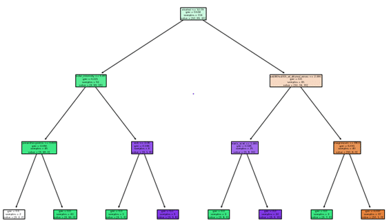
2.4 決定木の図

# The plot of first Decision Tree

_ = tree.plot_tree(rf.estimators_[0], feature_names=X.columns, filled=True)

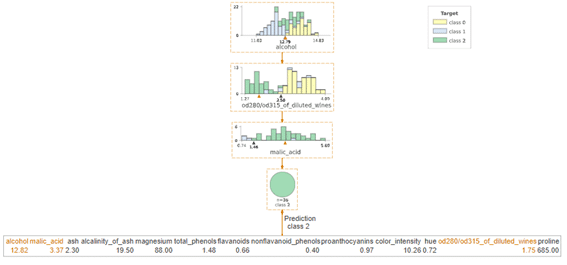
2.5 dtreeviz決定木の図

# dtreeviz decision tree

dtreeviz(rf.estimators_[0], X, y, feature_names=X.columns, target_name=”Target”)

対象データを作成します。

# random sample

X_ = wine.data[np.random.randint(0, len(wine.data)),:]

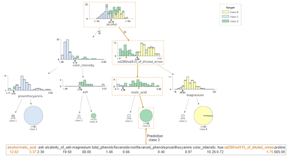
dtreeviz決定木の図　＋　対象データ

# dtreeviz decision tree with random sample

dtreeviz(rf.estimators_[0], X, y, feature_names=X.columns, X=X_, target_name=”Target”)

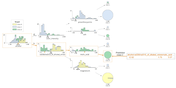
dtreeviz水平決定木の図

# Left-right dtreeviz decision tree

dtreeviz(rf.estimators_[0], X, y, feature_names=X.columns, orientation =’LR’, X=X_, target_name=”Target”)

対象データを注目してdtreeviz決定木の図

# dtreeviz decision tree with random sample + show_just_path

dtreeviz(rf.estimators_[0], X, y, feature_names=X.columns,

target_name=”Target”, orientation =’TD’,

X=X_, show_just_path=True)

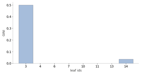
2.6 葉の純度

Random Forestの別れていった葉のデータの割合は予測の信頼性に影響します。分類の場合、葉の純度は多数派のターゲットクラス（ジニ、エントロピー）に基づいて計算されます。予測した結果の分散が小さい葉（回帰も含む）つまり分類が偏っている時（分類）は、はるかに信頼性の高い予測値です（回帰も含む）。

# Leaf node purity

viz_leaf_criterion(rf.estimators_[0], display_type = “plot”)

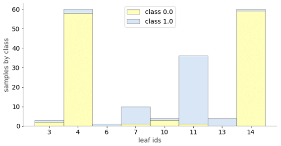
2.7 ターゲットクラスの分布

分類のための視覚化です。葉のサンプルからターゲットクラス値の分布を確認できます。

# Leaf node samples for classification

ctreeviz_leaf_samples(rf.estimators_[0], X, y)

担当者：HM

香川県高松市出身　データ分析にて、博士（理学）を取得後、自動車メーカー会社にてデータ分析に関わる。その後コンサルティングファームでデータ分析プロジェクトを歴任後独立　気が付けばデータ分析プロジェクトだけで５０以上担当

理化学研究所にて研究員を拝命中　応用数理学会所属

目次