eli5でモデルの解釈

1. eli5の概要

Eli5は「Explain Like I’m 5 (私が5歳だと思って説明して)」を略したスラングです。Eli5はscikit-learn、XGBoost、LightGBMなどの機械学習モデルを解釈するPythonライブラリです。

eli5は機械学習モデルを解釈する2つのレベルを提供します。

グローバルレベル：モデルの特徴量の重要さを説明します。

ローカルレベル：個々のサンプル予測を分析して、特定の予測が行われた理由を理解します。

2. 実験

環境：Google Colab

モデル解釈：eli5

ライブラリのインストール

!pip install eli5

ライブラリのインポート

import pandas as pd

import numpy as np

import sklearn

import eli5

2.1 回帰モデル

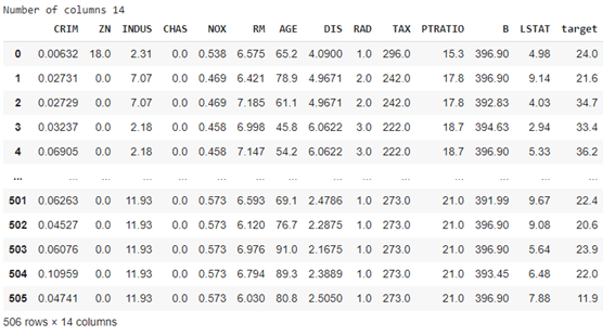
ボストン住宅価格データセットを読み込みます。

from sklearn.datasets import load_boston

boston = load_boston()

data = pd.DataFrame(np.c_[boston[‘data’], boston[‘target’]],

columns= np.append(boston[‘feature_names’], [‘target’]))

print(‘Number of columns’, len(data.columns))

data

学習とテストのデータを分けます。

from sklearn.model_selection import train_test_split

X = data.drop([‘target’], axis=1)

y = data[‘target’]

X_train, X_test, y_train, y_test = train_test_split(X, y, train_size=0.90, test_size=0.1, random_state=123, shuffle=True)

print(X_train.shape, X_test.shape, y_train.shape, y_test.shape)

(455, 13) (51, 13) (455,) (51,)

DecisionTreeRegressorのモデルを学習します。

from sklearn.tree import DecisionTreeRegressor

dtree = DecisionTreeRegressor(max_depth=4, max_leaf_nodes=250, max_features=”log2″)

dtree.fit(X_train, y_train)

print(“Train r2 : “, lr.score(X_train, y_train))

print(“Test r2 : “, lr.score(X_test, y_test))

Train r2 : 0.7511685217987627

Test r2 : 0.6412254020969461

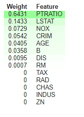
eli5でモデルの特徴量の重要を作成します。PTRATIOは一番重要な特徴量です。

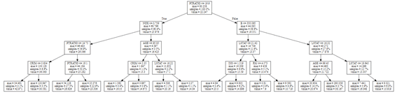
また、決定木のツリー図を表示します。

from eli5 import show_weights

show_weights(dtree, feature_names=boston.feature_names)

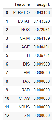
Pandasのデータフレームの結果を作成します。

from eli5.sklearn import explain_weights_sklearn

from eli5.formatters import format_as_dataframe, format_as_dataframes

explanation = explain_weights_sklearn(dtree, feature_names=boston.feature_names)

format_as_dataframe(explanation)

テキストの結果を作成することもできます。

from eli5.formatters import format_as_text

print(format_as_text(explanation))

Explained as: decision tree

Decision tree feature importances; values are numbers 0 <= x <= 1;

all values sum to 1.

0.6431 PTRATIO

0.1433 LSTAT

0.0729 NOX

0.0542 CRIM

0.0405 AGE

0.0358 B

0.0095 DIS

0.0007 RM

0 TAX

0 RAD

0 CHAS

0 INDUS

0 ZN

PTRATIO <= 19.900 (60.4%)

NOX <= 0.759 (56.9%)

PTRATIO <= 14.750 (6.6%)

CRIM <= 0.634 (3.1%) —> 42.97142857142858

CRIM > 0.634 (3.5%) —> 30.581250000000004

PTRATIO > 14.750 (50.3%)

PTRATIO <= 18.100 (27.5%) —> 26.926399999999987

PTRATIO > 18.100 (22.9%) —> 23.305769230769233

NOX > 0.759 (3.5%)

AGE <= 95.850 (1.3%)

CRIM <= 2.350 (0.4%) —> 16.55

CRIM > 2.350 (0.9%) —> 14.675

AGE > 95.850 (2.2%)

LSTAT <= 16.220 (1.1%) —> 20.160000000000004

LSTAT > 16.220 (1.1%) —> 14.039999999999997

PTRATIO > 19.900 (39.6%)

B <= 350.065 (11.6%)

LSTAT <= 21.420 (6.6%)

DIS <= 1.519 (0.4%) —> 25.3

DIS > 1.519 (6.2%) —> 14.896428571428569

LSTAT > 21.420 (5.1%)

RM <= 4.573 (0.4%) —> 7.9

RM > 4.573 (4.6%) —> 10.719047619047622

B > 350.065 (27.9%)

LSTAT <= 16.320 (15.2%)

AGE <= 99.450 (14.5%) —> 20.974242424242423

AGE > 99.450 (0.7%) —> 38.166666666666664

LSTAT > 16.320 (12.7%)

LSTAT <= 19.645 (5.9%) —> 16.048148148148147

LSTAT > 19.645 (6.8%) —> 10.91935483870968

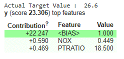
モデルのローカルの解釈します。y_testの一つのサンプルの予測を説明します。NOXとPTRATIOの特徴量はプラスの影響になっています。

from eli5 import show_prediction

print(“Actual Target Value : “, y_test.iloc[1])

show_prediction(dtree, X_test.iloc[1], feature_names=boston.feature_names, show_feature_values=True)

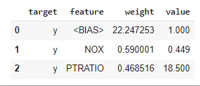
データフレームの結果を作成します。

from eli5.sklearn import explain_prediction

explanation = explain_prediction.explain_prediction_tree_regressor(dtree, X_test.iloc[1],

feature_names=boston.feature_names)

format_as_dataframe(explanation)

2.2 分類モデル

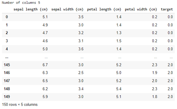
irisデータセットを読み込みます。

import pandas as pd

import numpy as np

from sklearn.datasets import load_iris

iris = load_iris()

data = pd.DataFrame(np.c_[iris[‘data’], iris[‘target’]],

columns= np.append(iris[‘feature_names’], [‘target’]))

print(‘Number of columns’, len(data.columns))

data

学習とテストのデータを分けます。

from sklearn.model_selection import train_test_split

X = data.drop([‘target’], axis=1)

y = data[‘target’]

X_train, X_test, y_train, y_test = train_test_split(X, y, train_size=0.90, test_size=0.1, random_state=123, shuffle=True)

print(X_train.shape, X_test.shape, y_train.shape, y_test.shape)

(135, 4) (15, 4) (135,) (15,)

DecisionTreeClassifierのモデルを学習します。

Accuracy, Confusion Matrix, Classification Reportを計算します。

from sklearn.tree import DecisionTreeClassifier

from sklearn.metrics import confusion_matrix, classification_report

dtree = DecisionTreeClassifier(max_depth=None, max_features=”log2″)

dtree.fit(X_train, y_train)

print(“Train Accuracy : %.2f”%dtree.score(X_train, y_train))

print(“Test Accuracy : %.2f”%dtree.score(X_test, y_test))

print()

print(“Confusion Matrix : “)

print(confusion_matrix(y_test, dtree.predict(X_test)))

print()

print(“Classification Report”)

print(classification_report(y_test, dtree.predict(X_test)))

Train Accuracy : 1.00

Test Accuracy : 0.93

Confusion Matrix :

[[4 0 0]

[0 4 1]

[0 0 6]]

Classification Report

precision recall f1-score support

0.0 1.00 1.00 1.00 4

1.0 1.00 0.80 0.89 5

2.0 0.86 1.00 0.92 6

accuracy 0.93 15

macro avg 0.95 0.93 0.94 15

weighted avg 0.94 0.93 0.93 15

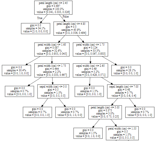
eli5でモデルの特徴量の重要を作成します。決定木のツリー図を表示します。

show_weights(dtree, feature_names=iris.feature_names,

show=[“feature_importances”, “decision_tree”, “method”, “description”])

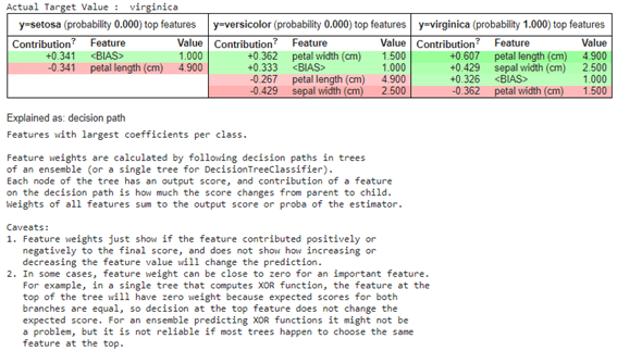
一つのサンプルの予測結果を説明します。Virginiceの予測結果はpetal lengthとsepal witdthで判断しました。

print(“Actual Target Value : “, iris.target_names[int(y_test.iloc[1])])

show_prediction(dtree,

X_test[:1],

feature_names=iris.feature_names,

targets=[0,1,2], target_names=iris.target_names,

show_feature_values=True,

show=[“targets”, “method”, “description”]

)

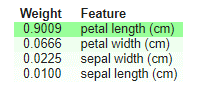
データフレームの結果を作成します。

from eli5.sklearn import explain_weights_sklearn

explanation = explain_weights_sklearn(dtree, feature_names=iris.feature_names, target_names=iris.feature_names)

from eli5.formatters import format_as_dataframe, format_as_dataframes

format_as_dataframe(explanation)

テキストの結果を作成します。

from eli5.formatters import format_as_text

print(format_as_text(explanation))

Explained as: decision tree

Decision tree feature importances; values are numbers 0 <= x <= 1;

all values sum to 1.

0.9009 petal length (cm)

0.0666 petal width (cm)

0.0225 sepal width (cm)

0.0100 sepal length (cm)

petal length (cm) <= 2.450 (34.1%) —> [1.000, 0.000, 0.000]

petal length (cm) > 2.450 (65.9%)

petal length (cm) <= 4.850 (32.6%)

petal width (cm) <= 1.650 (30.4%) —> [0.000, 1.000, 0.000]

petal width (cm) > 1.650 (2.2%)

petal width (cm) <= 1.750 (0.7%) —> [0.000, 0.000, 1.000]

petal width (cm) > 1.750 (1.5%)

sepal width (cm) <= 3.000 (0.7%) —> [0.000, 0.000, 1.000]

sepal width (cm) > 3.000 (0.7%) —> [0.000, 1.000, 0.000]

petal length (cm) > 4.850 (33.3%)

petal width (cm) <= 1.750 (5.2%)

sepal width (cm) <= 2.650 (1.5%) —> [0.000, 0.000, 1.000]

sepal width (cm) > 2.650 (3.7%)

sepal length (cm) <= 7.050 (3.0%)

petal length (cm) <= 5.050 (1.5%) —> [0.000, 1.000, 0.000]

petal length (cm) > 5.050 (1.5%)

petal width (cm) <= 1.550 (0.7%) —> [0.000, 0.000, 1.000]

petal width (cm) > 1.550 (0.7%) —> [0.000, 1.000, 0.000]

sepal length (cm) > 7.050 (0.7%) —> [0.000, 0.000, 1.000]

petal width (cm) > 1.750 (28.1%) —> [0.000, 0.000, 1.000]

担当者：KW
バンコクのタイ出身　データサイエンティスト
製造、マーケティング、財務、AI研究などの様々な業界にPSI生産管理、在庫予測・最適化分析、顧客ロイヤルティ分析、センチメント分析、SaaS、PaaS、IaaS、AI at the Edge の環境構築などのスペシャリスト

目次

1. eli5の概要

2. 実験

2.1 回帰モデル

2.2 分類モデル