星クラスター分析（Star Clustering）の解説

1. 星クラスター分析の概要

1.1 星クラスター分析のクラスター分析とは

星クラスター分析（Star Clustering）は、大まかに触発され、星系形成のプロセスに類似したクラスタリング手法です。その目的は、事前にクラスターの数を知る必要がない、クラスター作成します。

1.2 Star Clusteringのライブラリ

Star Clusteringのライブラリはpip installができないです。ただjosephius のgithub（下記のURL）からstar_clustering.pyをダウンロードすれば、star = StarCluster()のオブジェクトを作成して、星クラスター分析ができます。

https://github.com/josephius/star-clustering

2. 実験

環境：Colab

データセット：Sci-kit learnのirisはアヤメの種類と特徴量に関するデータセットで、3種類のアヤメの花弁と萼(がく)に関する特徴量について多数のデータです。

モデル：Star Clusteringのクラスター分析

2.1 環境設定

Star Clusteringのモジュールをダウンロードします。

import urllib

from urllib import request

img_src = “https://github.com/josephius/star-clustering/raw/master/star_clustering.py”

img_path = ‘star_clustering.py’

urllib.request.urlretrieve(img_src, img_path)

ライブラリのインストール

import numpy as np

import matplotlib.pyplot as plt

from mpl_toolkits.mplot3d import Axes3D

from sklearn.cluster import KMeans

from sklearn import datasets

from star_clustering import StarCluster

np.random.seed(5)

2.3 データロード

Irisのデータセットを読み込みます。

iris = datasets.load_iris()

X = iris.data

y = iris.target

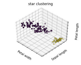
2.4 STAR CLUSTERINGの可視化

クラスタ数をあらかじめ設定しなくても、クラスタリングできます。二つのクラスターができました。

estimators = [(‘star_clustering_iris’, StarCluster())]

fignum = 1

titles = [‘Star Clustering’]

for name, est in estimators:

fig = plt.figure(fignum, figsize=(4, 3))

ax = Axes3D(fig, rect=[0, 0, .95, 1], elev=48, azim=134)

est.fit(X)

labels = est.labels_

ax.scatter(X[:, 3], X[:, 0], X[:, 2],

c=labels.astype(np.float), edgecolor=’k’)

ax.w_xaxis.set_ticklabels([])

ax.w_yaxis.set_ticklabels([])

ax.w_zaxis.set_ticklabels([])

ax.set_xlabel(‘Petal width’)

ax.set_ylabel(‘Sepal length’)

ax.set_zlabel(‘Petal length’)

ax.set_title(titles[fignum – 1])

ax.dist = 12

fignum = fignum + 1

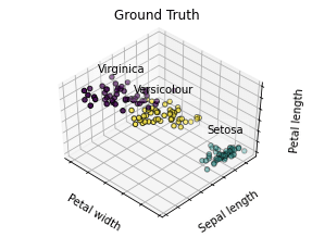
# Plot the ground truth

fig = plt.figure(fignum, figsize=(4, 3))

ax = Axes3D(fig, rect=[0, 0, .95, 1], elev=48, azim=134)

for name, label in [(‘Setosa’, 0),

(‘Versicolour’, 1),

(‘Virginica’, 2)]:

ax.text3D(X[y == label, 3].mean(),

X[y == label, 0].mean(),

X[y == label, 2].mean() + 2, name,

horizontalalignment=’center’,

bbox=dict(alpha=.2, edgecolor=’w’, facecolor=’w’))

# Reorder the labels to have colors matching the cluster results

y = np.choose(y, [1, 2, 0]).astype(np.float)

ax.scatter(X[:, 3], X[:, 0], X[:, 2], c=y, edgecolor=’k’)