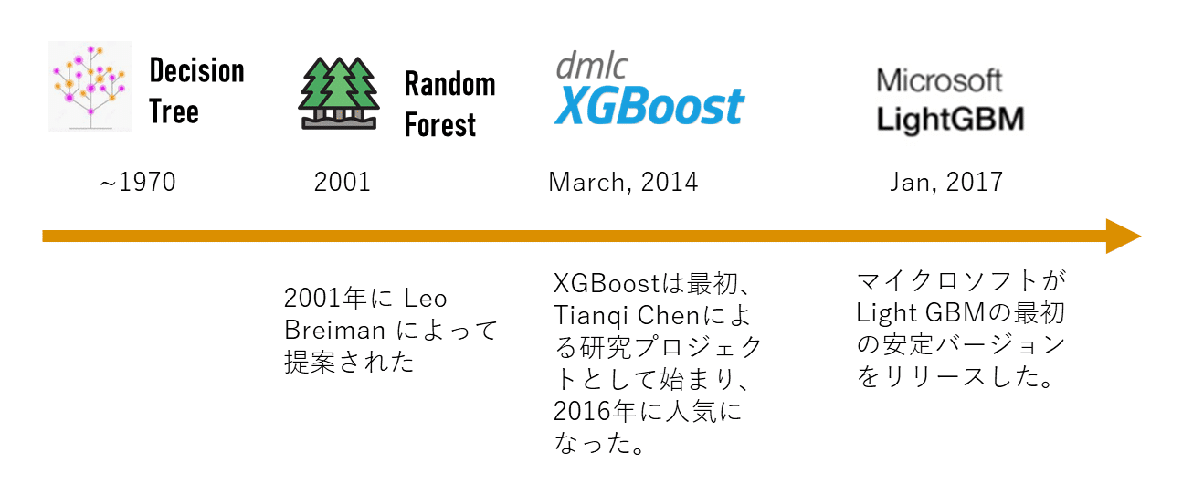
関連記事: 決定木分析、ランダムフォレスト、Xgboost、CatBoost
「勾配ブースティング」の開発は順調に進んでいます。 勾配ブースティングは、Kaggleで上位ランキングを取った半数以上もの勝者が勾配ブースティングを利用しました。 この記事では、Microsoft開発の「勾配ブースティング」のlightGBMを解説します。
目次
1. LightGBMとは
2. LightGBMの特徴
3. LightGBMのパラメーター
4. 実験・コード
__4.1 データ読み込み
__4.2 xgb
__4.3 lightgb
__4.4 モデル評価
1. LightGBMとは
LightGBM(読み:ライト・ジービーエム)決定木アルゴリズムに基づいた勾配ブースティング(Gradient Boosting)の機械学習フレームワークです。LightGBMは米マイクロソフト社2016年にリリースされました。前述した通り勾配ブースティングは複数の弱学習器(LightGBMの場合は決定木)を一つにまとめるアンサンブル学習の「ブースティング」を用いた手法です。
LightGBMは大規模なデータセットに対して計算コストを極力抑える工夫が施されています。この工夫により、多くのケースで他の機械学習手法と比較しても短時間でモデル訓練が行えます。
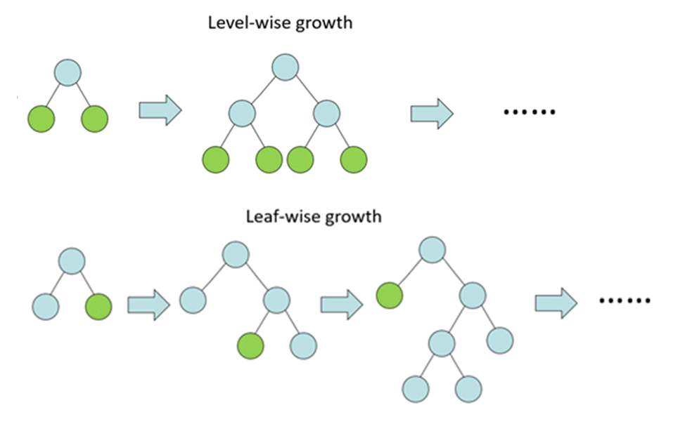
LightGBMはこの「Leaf-wise」という手法を採用しています。従来の「Level-wise」に比べてLightGBMが採用している「Leaf-wise」は訓練時間が短くなる傾向にあります。
2. LightGBMの特徴
モデル訓練に掛かる時間が短い
メモリ効率が高い
Leaf-Wiseのため推測精度が高い。
LightGBMは大規模データに適している手法
3. LightGBMのパラメーター
・booster [default=gbtree]
モデルのタイプを選択: gbtree: ツリーベースのモデル gblinear: 線形モデル
・silent [default=0]:
メッセージのモード:1=メッセージを表示しない 0 = メッセージを表示する
・nthread [デフォルトで利用可能なスレッドの最大数]
スレッド数の設定
・eta [default=0.3
GBMのlearning rate
各ステップの重みを縮小することにより、モデルをより堅牢にする
よく使用される値:0.01〜0.2
・min_child_weight [default=1]
過剰適合の制御に使用されます。値が大きすぎると、学習不足になる可能性があるため、CVを使用して調整する必要があります。
・max_depth [default=6]
ツリーの最大深度。
よく使用される値:3–10
・max_leaf_nodes
ツリー内のノードの最大数。
・gamma [default=0]
分割を行うために必要な最小損失削減を指定する。
・max_delta_step [default=0]
最大デルタステップでは、各ツリーの重み推定を許可します。 値が0に設定されている場合、制約がないこと。
・subsample [default=1]
各ツリーのランダムなサンプルの設定。値を小さくすると、オーバーフィッティングが防止されますが、小さすぎる値はアンダーフィッティングにつながる可能性があります。
・lambda [default=1]
L2正則化重み
・alpha [default=0]
L1正則化重み
・scale_pos_weight [default=1]
収束が速くなるように、クラスの不均衡が大きい場合は、0より大きい値を使用する必要がある
・objective [default=reg:linear]
binary:logistic –バイナリ分類のロジスティック回帰
multi:softmax – softmax目標を使用したマルチクラス分類
multi:softprob –softmaxと同じですが、各クラスに属する各データポイントの予測確率
・eval_metric [ default according to objective ]
rmse — root mean square error
mae — mean absolute error
logloss — negative log-likelihood
error — Binary classification error rate (0.5 threshold)
merror — Multiclass classification error rate
mlogloss — Multiclass logloss
auc: Area under the curve.
4. 実験・コード
概要:
データセット:学歴や出身などの経歴データをもとに年収が50Kドル以上かどうかが分類されたデータセット
https://www.kaggle.com/wenruliu/adult-income-dataset
モデル: xgboost vs lightgbm
モデル評価:Accuracy AUC 実行時間
4.1 データ読み込み
#ライブラリのインポート
import numpy as np
import pandas as pd
from pandas import Series, DataFrame

import lightgbm as lgbm
import xgboost as xgb

#データ読み込み
df=pd.read_csv('/content/drive/My Drive/dataset/income.csv',header=None)

#カラム名の変更
df.columns=['age','work_class','fnl_wgt','education','education-num','marital_Status',
'occupation','relationship','race','sex','capital_gain','capital_loss','hours_per_week',
'native_country','Income']

df.head()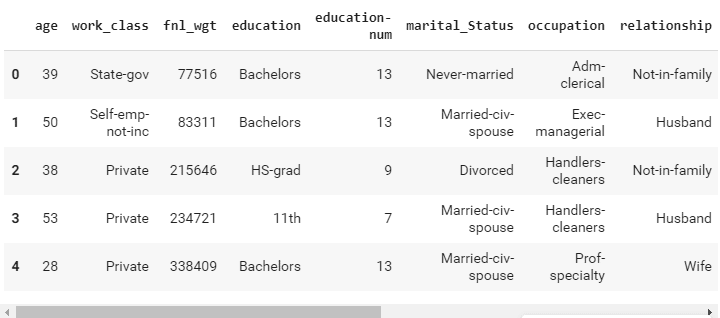
# LabelEncoding
from sklearn.preprocessing import LabelEncoder,OneHotEncoder
l=LabelEncoder()
l.fit(df.Income)
df.Income=Series(l.transform(df.Income))
df.Income.value_counts()
0 24720
1 7841
Name: Income, dtype: int64
#One_Hot_Encoding
one_hot_work_class=pd.get_dummies(df.work_class)
one_hot_education=pd.get_dummies(df.education)
one_hot_marital_Status=pd.get_dummies(df.marital_Status)
one_hot_occupation=pd.get_dummies(df.occupation)
one_hot_relationship=pd.get_dummies(df.relationship)
one_hot_race=pd.get_dummies(df.race)
one_hot_sex=pd.get_dummies(df.sex)
one_hot_native_country=pd.get_dummies(df.native_country)

#categorical features削除
df.drop(['work_class','education','marital_Status','occupation','relationship',
'race','sex','native_country'],axis=1,inplace=True)

#Merging one hotの結合
df=pd.concat([df,one_hot_work_class,one_hot_education,one_hot_marital_Status,
one_hot_occupation,one_hot_relationship,
one_hot_race,one_hot_sex,one_hot_native_country],axis=1)

_, i = np.unique(df.columns, return_index=True) #重複データ削除
df=df.iloc[:, i]
#x yの設定
x=df.drop('Income',axis=1)
y=df.Income

#欠損値処理
y.fillna(y.mode()[0],inplace=True)

#学習とテストを分ける
from sklearn.model_selection import train_test_split
x_train,x_test,y_train,y_test=train_test_split(x,y,test_size=.3)
4.2 xgb
#変数設定
dtrain=xgb.DMatrix(x_train,label=y_train)
dtest=xgb.DMatrix(x_test)

#パラメータ設定
parameters={'max_depth':7, 'silent':1,'objective':'binary:logistic','eval_metric':'auc','learning_rate':.05}

#学習
num_round=50
from datetime import datetime
start = datetime.now()
xg=xgb.train(parameters,dtrain,num_round)
stop = datetime.now()
execution_time_xgb = stop-start
execution_time_xgb

#予測
ypred=xg.predict(dtest)
ypred
for i in range(0,9769):
if ypred[i]>=.5: # setting threshold to .5
ypred[i]=1
else:
ypred[i]=0

#モデル評価
from sklearn.metrics import accuracy_score
accuracy_xgb = accuracy_score(y_test,ypred)
accuracy_xgb
0.8689732828334528
4.3 lightgb
#データ読み込み
train_data=lgbm.Dataset(x_train,label=y_train)

#パラメータ設定
param = {'num_leaves':150, 'objective':'binary','max_depth':7,'learning_rate':.05,'max_bin':200}
param['metric'] = ['auc', 'binary_logloss']

#学習
num_round=50
start=datetime.now()
lgbm=lgbm.train(param,train_data,num_round)
stop=datetime.now()

execution_time_lgbm = stop-start
execution_time_lgbm
#予測 ypred2=lgbm.predict(x_test) ypred2[0:5] # showing first 5 predictions for i in range(0,9769): if ypred2[i]>=.5: # setting threshold to .5 ypred2[i]=1 else: ypred2[i]=0
array([0.02714056, 0.04078569, 0.9078372 , 0.60302779, 0.27518461])
#モデル評価
accuracy_lgbm = accuracy_score(ypred2,y_test)
accuracy_lgbm
y_test.value_counts()

from sklearn.metrics import roc_auc_score
#calculating roc_auc_score for xgboost
auc_xgb = roc_auc_score(y_test,ypred)
auc_xgb
0.7729192155105222
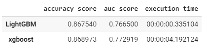
4.4 モデル評価
#light gbmのroc_auc_score
auc_lgbm = roc_auc_score(y_test,ypred2)
auc_lgbm_comparison_dict = {'accuracy score':(accuracy_lgbm,accuracy_xgb),'auc score':(auc_lgbm,auc_xgb),'execution time':(execution_time_lgbm,execution_time_xgb)}

#結果の表
comparison_df = DataFrame(auc_lgbm_comparison_dict)
comparison_df.index= ['LightGBM','xgboost']
comparison_df